
Goal: Graduate Student Demonstration of Ensemble Methods
The Gradient Boosting Workflow
Math Behind the Gradient Boosting
What are Ensemble Methods
Ensemble methods are machine learning techniques that use multiple models to improve the accuracy of predictions. These methods can be more effective than using a single model alone. There are several types of ensemble methods which include stacking, bagging, boosting, and more. Boosting, which is one type of ensemble method, involves building a series of models sequentially to correct errors made by the previous models.
What is Gradient Boosting? 

Gradient Boosting is a specific type of boosting method that uses gradient descent to optimize the model’s performance. Gradient Boosting is used in supervised learning tasks such as regression and classification problems. The “gradient” refers to the optimization process used to minimize the errors made by each model in the sequence. Specifically, Gradient Boosting uses gradient descent to find the optimal direction to update the model’s parameters. The subsequent models in gradient boosting rely on the previous model, allowing the algorithm to learn more effectively and generate more accurate predictions. However, Gradient Boosting comes with increased cost and time complexity compared to other machine learning algorithms because of its iterative mechanism, hyperparameter tuning, and memory requirements.
The Gradient Boosting Workflow

The mechanism of Gradient Boosting begins by selecting a weak learner, which is typically a simple model that is not very accurate. Gradient Boosting uses the decision tree structure for its weak learner, which resembles a tree-like model that makes a sequence of decisions to arrive at a final prediction. Once the weak learner is selected, it is fit to the data to make a prediction. The error (residual) between the predicted and actual values is then calculated. This error represents the gap between the current model’s predictions and the true outcomes and is used to adjust the weights of the observations in the dataset. The updated weights are then used to build a new weak learner, which is added to the previous one to form a more accurate, stronger model. This process of building a new weak learner and updating the weights is repeated multiple times, with each iteration improving the accuracy of the model.
Let’s use Gradient Boosting for the following training data to predict CO2 emissions.
| Car type | fuel type | cylinders | co2 emission (g/KM) |
|---|---|---|---|
| 2 Door | Gasoline | 6 | 230 |
| 4 Door | Electric | 4 | 75 |
| 4 Door | Gasoline | 8 | 285 |
| 2 Door | Gasoline | 4 | 195 |
| 4 Door | Electric | 4 | 85 |
| 2 Door | Electric | 4 | 100 |
To begin predicting CO2 emissions for vehicles, the first step is to calculate the average CO2 emission, which is currently at 175 g/km. The next step involves using Gradient Boosting to build a tree based on the errors from the previous tree. The errors (residuals) are calculated as the difference between the observed values and predicted values.
| Car Type | Fuel type | cylinders | co2 Emission (g/km) | pseudo residual |
|---|---|---|---|---|
| 2 Door | Gasoline | 6 | 230 | 55 |
| 4 Door | Electric | 4 | 75 | -100 |
| 4 Door | Gasoline | 8 | 285 | 110 |
| 2 Door | Gasoline | 4 | 195 | 20 |
| 4 Door | Electric | 4 | 85 | -90 |
| 2 Door | Electric | 4 | 100 | -75 |
After obtaining the residuals for each value, a tree is developed based on the available features such as Car Type, Fuel Type, and Cylinders to determine the residuals.
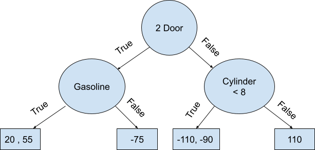
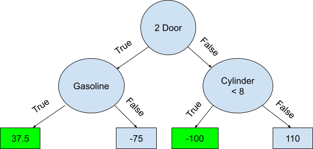
Once the residuals with two values in their leaf are calculated, the average of the residuals is replaced. This is known as the “majority voting” technique.
Starting with the initial prediction of 175 g/km, the leaf with a CO2 emission value of 110 g/km is used to predict the final value of 285 g/km, which is higher than the expected value. It means that our model has a high bias and low variance. High bias means that our model is not complex enough to capture the true relationship between the independent variables and the target variable, and as a result, it consistently underestimates or overestimates the target variable. This is usually caused by a lack of features, a poor choice of hyperparameters, or a small dataset. Low variance means that our model is not sensitive to the noise in the training data and can generalize well to unseen data. A model with high variance would have fit the training data very closely, including the noise in the data, and would not have generalized well to new data. Therefore the creation of a generalized model with both low variance and low bias is important for achieving accurate and reliable predictions.
In order to prevent overfitting and underfitting, the Gradient Boosting algorithm uses a hyperparameter called Learning Rate to scale the contribution from the new tree. The Learning Rate has a scale between 0 and 1, and it determines the step size at which the algorithm learns from the mistakes made by the previous tree in the ensemble. A lower Learning Rate results in slower learning, but the final model generalizes better and avoids overfitting, whereas a higher Learning Rate leads to faster learning but may result in overfitting and poor performance. In this example, a Learning Rate of 0.1 is assigned to the model, resulting in a predicted CO2 emission of 175 + (0.1 x 110) equals 186 g/km, which is slightly better than the original prediction of 175 g/km.
This procedure is repeated, and new residuals are created using the new predicted values. The residuals shrink as more trees are added to the model, and as additional trees are added, the residuals get smaller. This procedure continues until the maximum number of trees is given, or until adding more trees does not substantially lower the size of the residuals.
Math Behind the Gradient Boosting

We will use mathematical steps to build an ensemble of trees on Gradient Boosting:
STEP 1: Inserting Data ![]()
- We are given the 𝑛 input data where 𝑥𝟷 is a vector of the independent variables and 𝑦𝟷 is our target variable.
STEP 2: For 𝑚 = 𝟷 to 𝑀
- In this step ensemble process starts with a loop where 𝑚 indicates the number of trees
STEP 3: We calculate the Loss Function
- Loss Function: 𝐿(𝑦₁, 𝐹(𝑥))
- Also, we need to assign our Loss Function, which in our context we used Pseudo Residual.
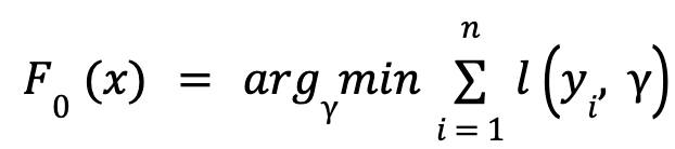
- We initialize the model with a constant value:

- As previously stated, 𝐿 represents our loss function and Gamma (𝛾) is our predicted value and 𝐹₀(𝑥) is our base model. Our objective is to optimize our model by utilizing the loss function, which takes the form of a Pseudo Residual.
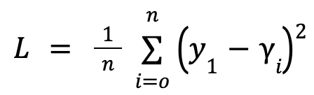
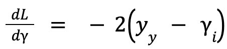
- Since our independent variable is continuous, the Loss Function is:

- This function calculates the squared difference between predicted values and actual values for each row, and then takes the mean of these squared differences to obtain the overall loss.
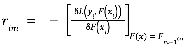
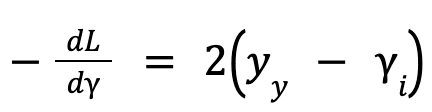
- Then we take the derivative of the Loss Function:
-

- 𝐿 = (𝑦₁ – 𝛾₁)2


- This function will calculate the residual of each row. The negative sign indicates the direction of the steepest ascent. In the context of optimization, the objective is typically to minimize the loss function.
-
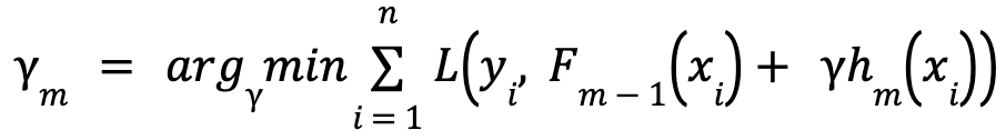
- As stated earlier, it is common to have multiple training instances that end up in the same leaf node, which means that the predicted values for that particular leaf node should be an average of those values:

- In this function ℎ𝑚(𝑥𝑖) refers to a decision tree that is trained on the residuals and the m parameter indicates the number of trees in the gradient algorithm.
FINAL STEP: The next step is to update the predictions of the current ensemble of learners by adding the output of the new base learner and multiplying by a learning rate after obtaining the optimal values of the base learner:
𝐹𝑚(𝑥𝑖) = 𝐹𝑚-𝟷 (𝑥𝑖) + 𝑙𝑒𝑎𝑟𝑛𝑖𝑛𝑔 𝑟𝑎𝑡𝑒 * ℎ𝑚(𝑥𝑖)
After updating the predictions of the current ensemble, the algorithm replicates the same procedure by finding the optimal value of the next base learner to reduce the loss function on the residuals and adding it to the ensemble. This process is repeated until either the maximum number of trees is provided or until increasing the number of trees does not significantly reduce the size of the residuals.
Summary
In conclusion, we looked at the math underlying gradient boosting, a potent and reliable machine learning strategy that combines a number of poor predictive models into a strong one. Despite the fact that the algorithm may appear complex at first glance, It is worth understanding the steps involved in order to fully understand how it works. By using Gradient Boosting, we can handle complex datasets and achieve high accuracy in our predictions. Whether you are a data scientist, a researcher, or just someone interested in the world of machine learning, understanding Gradient Boosting can be a valuable asset. So do not be intimidated by the math – take the time to learn this technique and see what it can do for your own work.
The University of San Diego’s Master of Science in Applied Data Science (MS-ADS) program offers a robust curriculum that focuses both on the technical and soft skills required to become a successful data scientist. USD’s MS-ADS online program ensures that our students graduate with the data scientist skills needed to succeed in the workforce and understand this skill set is not limited to strictly technical training. USD’s MS-ADS online program was developed by industry experts who have firsthand knowledge of the practical skills required and have designed its courses to reflect this ever-evolving industry.
Icon Credit
Algorithm icons created by juicy_fish – Flaticon